Exploratory Data Analysis on Car prices Prediction Dataset

Submitted by

Shah Nawaz - (lead)
Saleha Attiq - (co-lead)
Rabia Attiq
Muhammad Abdullah
Naveed ul Mustafa
Khurram Shehzad
Ali Husnain
Karan Kumar
Muhammad Abdullah
Ali Hamza

on 20-08-2022

1- Project Description

A company is planning to build a manufacturing unit. They have gathered car price data from an automobile consulting company of that particular region to understand the factors on which the pricing of cars depends. The company wants to know:

Which variables are significant in predicting the price of a car
How well those variables describe the price of a car

2- Objective

To reach an informed business decision and capturing the market following factors need to carefully studied through EDA:

To find out correlation of price with the available independent variables.
To plan the strategy for choosing the car design and features which are popular in this market based on the data set.
To see the trend of price and accordingly set the prices of variants.

3- Methodology

Overview of the data
Checking shape, number of columns and missing values
Check for duplicate rows and drop if insignificant with respect to data size
Drop unnecssary columns with redundant or meaningless values.
Identifying Unique values in all columns
Detecting if there is any pseudo Unique or invalid entries in the columns. If any convert into Null value
Data type casting.
Replace the Null values with the mean.
Check the outlier values and treat them.
Data visualisation of the each categorical and numerical feature using barplot, boxplot, histograms, scatter plot, maps and line graphs.
Find out the Correlation

Step_1 Importing important libraries

# Import Libraries
import numpy as np
import pandas as pd
import matplotlib.pyplot as plt
import seaborn as sns

Step_2 Overview of dataset

Import Dataset

# Import Dataset
df = pd.read_csv("car_price_prediction.csv")
df.head()

	ID	Price	Levy	Manufacturer	Model	Prod. year	Category	Leather interior	Fuel type	Engine volume	Mileage	Cylinders	Gear box type	Drive wheels	Doors	Wheel	Color	Airbags
0	45654403	13328	1399	LEXUS	RX 450	2010	Jeep	Yes	Hybrid	3.5	186005 km	6.0	Automatic	4x4	04-May	Left wheel	Silver	12
1	44731507	16621	1018	CHEVROLET	Equinox	2011	Jeep	No	Petrol	3	192000 km	6.0	Tiptronic	4x4	04-May	Left wheel	Black	8
2	45774419	8467	-	HONDA	FIT	2006	Hatchback	No	Petrol	1.3	200000 km	4.0	Variator	Front	04-May	Right-hand drive	Black	2
3	45769185	3607	862	FORD	Escape	2011	Jeep	Yes	Hybrid	2.5	168966 km	4.0	Automatic	4x4	04-May	Left wheel	White	0
4	45809263	11726	446	HONDA	FIT	2014	Hatchback	Yes	Petrol	1.3	91901 km	4.0	Automatic	Front	04-May	Left wheel	Silver	4

Check the Data Shape

It is a important step.
First step to start EDA.

# Data Shape in terms of Row and columns
print('The number of rows are: ', df.shape[0])
print('The number of columns are: ', df.shape[1])

The number of rows are:  19237
The number of columns are:  18

Structure of Dataset

In this step we are seeing the structure of Dataset.
After running a code df.info() we will sees the data type and number of Non-Null values.

# Structure of the data
df.info()

<class 'pandas.core.frame.DataFrame'>
RangeIndex: 19237 entries, 0 to 19236
Data columns (total 18 columns):
 #   Column            Non-Null Count  Dtype  
---  ------            --------------  -----  
 0   ID                19237 non-null  int64  
 1   Price             19237 non-null  int64  
 2   Levy              19237 non-null  object 
 3   Manufacturer      19237 non-null  object 
 4   Model             19237 non-null  object 
 5   Prod. year        19237 non-null  int64  
 6   Category          19237 non-null  object 
 7   Leather interior  19237 non-null  object 
 8   Fuel type         19237 non-null  object 
 9   Engine volume     19237 non-null  object 
 10  Mileage           19237 non-null  object 
 11  Cylinders         19237 non-null  float64
 12  Gear box type     19237 non-null  object 
 13  Drive wheels      19237 non-null  object 
 14  Doors             19237 non-null  object 
 15  Wheel             19237 non-null  object 
 16  Color             19237 non-null  object 
 17  Airbags           19237 non-null  int64  
dtypes: float64(1), int64(4), object(13)
memory usage: 2.6+ MB

Step_3 Cleaning of Data

Rename Columns as a good practice

df = df.rename(columns={"Prod. year": "Prod_year",
 "Leather interior": "Leather_interior" , 
"Fuel type": "Fuel_type" , "Engine volume": "Engine_volume" , 
"Gear box type": "Gear_box_type" , "Drive wheels": "Drive_wheels"})

# Columns of DataFrame
df.columns

Index(['ID', 'Price', 'Levy', 'Manufacturer', 'Model', 'Prod_year', 'Category',
       'Leather_interior', 'Fuel_type', 'Engine_volume', 'Mileage',
       'Cylinders', 'Gear_box_type', 'Drive_wheels', 'Doors', 'Wheel', 'Color',
       'Airbags'],
      dtype='object')

Dealing with duplicates

# Checking the duplicates
df.duplicated().sum()

# Dropping the duplicates
df = df.drop_duplicates()

# Again checking the duplicates
df.duplicated().sum()

Dropping unncessary columns

df = df.iloc[: , 1:]
df.head()
# ID column is dropped
# By looking it the columns ID does not have any meaningful value

	Price	Levy	Manufacturer	Model	Prod_year	Category	Leather_interior	Fuel_type	Engine_volume	Mileage	Cylinders	Gear_box_type	Drive_wheels	Doors	Wheel	Color	Airbags
0	13328	1399	LEXUS	RX 450	2010	Jeep	Yes	Hybrid	3.5	186005 km	6.0	Automatic	4x4	04-May	Left wheel	Silver	12
1	16621	1018	CHEVROLET	Equinox	2011	Jeep	No	Petrol	3	192000 km	6.0	Tiptronic	4x4	04-May	Left wheel	Black	8
2	8467	-	HONDA	FIT	2006	Hatchback	No	Petrol	1.3	200000 km	4.0	Variator	Front	04-May	Right-hand drive	Black	2
3	3607	862	FORD	Escape	2011	Jeep	Yes	Hybrid	2.5	168966 km	4.0	Automatic	4x4	04-May	Left wheel	White	0
4	11726	446	HONDA	FIT	2014	Hatchback	Yes	Petrol	1.3	91901 km	4.0	Automatic	Front	04-May	Left wheel	Silver	4

Now unique value of every column will be checked and listed below those which required treatment. This step is necessary to find out that:

Whether the column has wrong unique value due to any spelling mistakes
Whether the column has abnormal unique value which does not correspond to that data column

# check if there zero in price
any(df.Price==0)

False

# check if there any negative number in price
any(df.Price<0)

False

df['Levy'].unique()
# This command helped us itdentifying "-" psuedo unique value in Levy column

array(['1399', '1018', '-', '862', '446', '891', '761', '751', '394',
       '1053', '1055', '1079', '810', '2386', '1850', '531', '586',
       '1249', '2455', '583', '1537', '1288', '915', '1750', '707',
       '1077', '1486', '1091', '650', '382', '1436', '1194', '503',
       '1017', '1104', '639', '629', '919', '781', '530', '640', '765',
       '777', '779', '934', '769', '645', '1185', '1324', '830', '1187',
       '1111', '760', '642', '1604', '1095', '966', '473', '1138', '1811',
       '988', '917', '1156', '687', '11714', '836', '1347', '2866',
       '1646', '259', '609', '697', '585', '475', '690', '308', '1823',
       '1361', '1273', '924', '584', '2078', '831', '1172', '893', '1872',
       '1885', '1266', '447', '2148', '1730', '730', '289', '502', '333',
       '1325', '247', '879', '1342', '1327', '1598', '1514', '1058',
       '738', '1935', '481', '1522', '1282', '456', '880', '900', '798',
       '1277', '442', '1051', '790', '1292', '1047', '528', '1211',
       '1493', '1793', '574', '930', '1998', '271', '706', '1481', '1677',
       '1661', '1286', '1408', '1090', '595', '1451', '1267', '993',
       '1714', '878', '641', '749', '1511', '603', '353', '877', '1236',
       '1141', '397', '784', '1024', '1357', '1301', '770', '922', '1438',
       '753', '607', '1363', '638', '490', '431', '565', '517', '833',
       '489', '1760', '986', '1841', '1620', '1360', '474', '1099', '978',
       '1624', '1946', '1268', '1307', '696', '649', '666', '2151', '551',
       '800', '971', '1323', '2377', '1845', '1083', '694', '463', '419',
       '345', '1515', '1505', '2056', '1203', '729', '460', '1356', '876',
       '911', '1190', '780', '448', '2410', '1848', '1148', '834', '1275',
       '1028', '1197', '724', '890', '1705', '505', '789', '2959', '518',
       '461', '1719', '2858', '3156', '2225', '2177', '1968', '1888',
       '1308', '2736', '1103', '557', '2195', '843', '1664', '723',
       '4508', '562', '501', '2018', '1076', '1202', '3301', '691',
       '1440', '1869', '1178', '418', '1820', '1413', '488', '1304',
       '363', '2108', '521', '1659', '87', '1411', '1528', '3292', '7058',
       '1578', '627', '874', '1996', '1488', '5679', '1234', '5603',
       '400', '889', '3268', '875', '949', '2265', '441', '742', '425',
       '2476', '2971', '614', '1816', '1375', '1405', '2297', '1062',
       '1113', '420', '2469', '658', '1951', '2670', '2578', '1995',
       '1032', '994', '1011', '2421', '1296', '155', '494', '426', '1086',
       '961', '2236', '1829', '764', '1834', '1054', '617', '1529',
       '2266', '637', '626', '1832', '1016', '2002', '1756', '746',
       '1285', '2690', '1118', '5332', '980', '1807', '970', '1228',
       '1195', '1132', '1768', '1384', '1080', '7063', '1817', '1452',
       '1975', '1368', '702', '1974', '1781', '1036', '944', '663', '364',
       '1539', '1345', '1680', '2209', '741', '1575', '695', '1317',
       '294', '1525', '424', '997', '1473', '1552', '2819', '2188',
       '1668', '3057', '799', '1502', '2606', '552', '1694', '1759',
       '1110', '399', '1470', '1174', '5877', '1474', '1688', '526',
       '686', '5908', '1107', '2070', '1468', '1246', '1685', '556',
       '1533', '1917', '1346', '732', '692', '579', '421', '362', '3505',
       '1855', '2711', '1586', '3739', '681', '1708', '2278', '1701',
       '722', '1482', '928', '827', '832', '527', '604', '173', '1341',
       '3329', '1553', '859', '167', '916', '828', '2082', '1176', '1108',
       '975', '3008', '1516', '2269', '1699', '2073', '1031', '1503',
       '2364', '1030', '1442', '5666', '2715', '1437', '2067', '1426',
       '2908', '1279', '866', '4283', '279', '2658', '3015', '2004',
       '1391', '4736', '748', '1466', '644', '683', '2705', '1297', '731',
       '1252', '2216', '3141', '3273', '1518', '1723', '1588', '972',
       '682', '1094', '668', '175', '967', '402', '3894', '1960', '1599',
       '2000', '2084', '1621', '714', '1109', '3989', '873', '1572',
       '1163', '1991', '1716', '1673', '2562', '2874', '965', '462',
       '605', '1948', '1736', '3518', '2054', '2467', '1681', '1272',
       '1205', '750', '2156', '2566', '115', '524', '3184', '676', '1678',
       '612', '328', '955', '1441', '1675', '3965', '2909', '623', '822',
       '867', '3025', '1993', '792', '636', '4057', '3743', '2337',
       '2570', '2418', '2472', '3910', '1662', '2123', '2628', '3208',
       '2080', '3699', '2913', '864', '2505', '870', '7536', '1924',
       '1671', '1064', '1836', '1866', '4741', '841', '1369', '5681',
       '3112', '1366', '2223', '1198', '1039', '3811', '3571', '1387',
       '1171', '1365', '1531', '1590', '11706', '2308', '4860', '1641',
       '1045', '1901'], dtype=object)

# Replacing "-" with null value in levy column
df['Levy'] = df['Levy'].replace('-', np.nan)
df['Wheel'] = df['Wheel'].str.replace('Left wheel','Left-hand drive')

df['Engine_volume'].unique()
# All unique values visible and it gives us an idea to split the column into two parts.
# One: Engine Volume and Other: Turbo Feature

array(['3.5', '3', '1.3', '2.5', '2', '1.8', '2.4', '4', '1.6', '3.3',
       '2.0 Turbo', '2.2 Turbo', '4.7', '1.5', '4.4', '3.0 Turbo',
       '1.4 Turbo', '3.6', '2.3', '1.5 Turbo', '1.6 Turbo', '2.2',
       '2.3 Turbo', '1.4', '5.5', '2.8 Turbo', '3.2', '3.8', '4.6', '1.2',
       '5', '1.7', '2.9', '0.5', '1.8 Turbo', '2.4 Turbo', '3.5 Turbo',
       '1.9', '2.7', '4.8', '5.3', '0.4', '2.8', '3.2 Turbo', '1.1',
       '2.1', '0.7', '5.4', '1.3 Turbo', '3.7', '1', '2.5 Turbo', '2.6',
       '1.9 Turbo', '4.4 Turbo', '4.7 Turbo', '0.8', '0.2 Turbo', '5.7',
       '4.8 Turbo', '4.6 Turbo', '6.7', '6.2', '1.2 Turbo', '3.4',
       '1.7 Turbo', '6.3 Turbo', '2.7 Turbo', '4.3', '4.2', '2.9 Turbo',
       '0', '4.0 Turbo', '20', '3.6 Turbo', '0.3', '3.7 Turbo', '5.9',
       '5.5 Turbo', '0.2', '2.1 Turbo', '5.6', '6', '0.7 Turbo',
       '0.6 Turbo', '6.8', '4.5', '0.6', '7.3', '0.1', '1.0 Turbo', '6.3',
       '4.5 Turbo', '0.8 Turbo', '4.2 Turbo', '3.1', '5.0 Turbo', '6.4',
       '3.9', '5.7 Turbo', '0.9', '0.4 Turbo', '5.4 Turbo', '0.3 Turbo',
       '5.2', '5.8', '1.1 Turbo'], dtype=object)

# Feature Engineering in engine volume column
df[['Engine_volume', 'Turbo_feature']] = df['Engine_volume'].str.split(' ',
 expand=True)

# Adding values of Turbo_feature
df['Turbo_feature'] = df['Turbo_feature'].map({'Turbo': True, 
None: False})

df['Mileage'].unique()
df['Mileage'].value_counts()
# This shows first we need to change its data type and then replace '0' with Null value for further correction.

0 km         714
200000 km    181
150000 km    159
160000 km    120
180000 km    117
            ... 
100563 km      1
354300 km      1
21178 km       1
110539 km      1
186923 km      1
Name: Mileage, Length: 7687, dtype: int64

# Changing the 0 km to null value
df['Mileage'] = df['Mileage'].replace('0 km', np.nan)

df['Doors'].unique()
# this command helped us itendifying that type casting will be required afterwards

array(['04-May', '02-Mar', '>5'], dtype=object)

Dealing with null values

Now, we run a code to see the number of missing values in a single column.
After seeing the number of values we have to replace it with its mean or we can drop it.
We check the precentages of null values and then decide.
If percentage is low we can replace it with mean or if high we can drop it.

# Finding the missing values in the dataframe
df.isnull().sum()

Price                  0
Levy                5709
Manufacturer           0
Model                  0
Prod_year              0
Category               0
Leather_interior       0
Fuel_type              0
Engine_volume          0
Mileage              714
Cylinders              0
Gear_box_type          0
Drive_wheels           0
Doors                  0
Wheel                  0
Color                  0
Airbags                0
Turbo_feature          0
dtype: int64

# Percentage of missing values in each column
null = df.isnull().sum()/df.shape[0]*100
null

Price                0.000000
Levy                30.168041
Manufacturer         0.000000
Model                0.000000
Prod_year            0.000000
Category             0.000000
Leather_interior     0.000000
Fuel_type            0.000000
Engine_volume        0.000000
Mileage              3.772987
Cylinders            0.000000
Gear_box_type        0.000000
Drive_wheels         0.000000
Doors                0.000000
Wheel                0.000000
Color                0.000000
Airbags              0.000000
Turbo_feature        0.000000
dtype: float64

# Bar graph of percentage of missing values in each column
plt.figure(figsize=(20,10))
sns.barplot(null.index, null.values)
plt.xlabel('Features', fontsize=12)
plt.ylabel('Percentage of missing values', fontsize=12)
plt.show()

c:\Users\WASIF\AppData\Local\Programs\Python\Python310\lib\site-packages\seaborn\_decorators.py:36: FutureWarning: Pass the following variables as keyword args: x, y. From version 0.12, the only valid positional argument will be `data`, and passing other arguments without an explicit keyword will result in an error or misinterpretation.
  warnings.warn(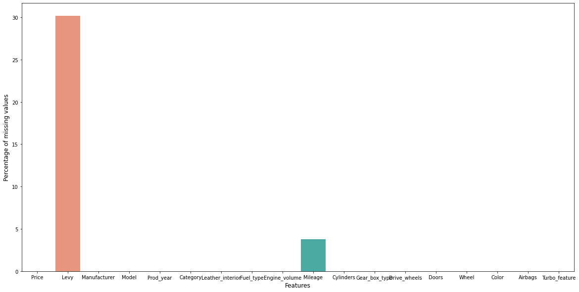

Step_4 Type Casting and Replacing Null

Perform type casting to further treat them.

# Changing data type of levy column
df['Levy'] = df['Levy'].astype(float)

# Droping Km in Mileage column to convert it to numeric
df['Mileage'] = df['Mileage'].str.replace('km', '')

# Convert Mileage column to numeric
df['Mileage'] = pd.to_numeric(df['Mileage'])
# Now again checking the data type of Mileage column
df[['Mileage','Levy']].dtypes

Mileage    float64
Levy       float64
dtype: object

We can see that the percentage of missing values in Levy and Mileage column is low.

# Replacing missing values in Mileage column with mean value
df['Mileage'].fillna(df['Mileage'].mean(), inplace=True)

# Replacing missing values in Levy column with mean value
df['Levy'].fillna(df['Levy'].mean(), inplace=True)

# Now again checking the number of missing values in each column
df.isnull().sum()

Price               0
Levy                0
Manufacturer        0
Model               0
Prod_year           0
Category            0
Leather_interior    0
Fuel_type           0
Engine_volume       0
Mileage             0
Cylinders           0
Gear_box_type       0
Drive_wheels        0
Doors               0
Wheel               0
Color               0
Airbags             0
Turbo_feature       0
dtype: int64

Treating door column.

It has value in ‘04-May’ it means that the car has four doors, ‘02-Mar’ means two doors and ‘>5’ mean more than 5 doors.
We changing it by the following codes;

# Repalcing -may and -mar with space in door column
df['Doors'] = df['Doors'].str.replace('-May', ' ')
df['Doors'] = df['Doors'].str.replace('-Mar', ' ')
df['Doors'] = df['Doors'].str.replace('>5', '6')
df['Doors'] = pd.to_numeric(df['Doors'])
df['Doors'].unique()

array([4, 2, 6], dtype=int64)

Treating Leather_interior column

Converting it into boolean type

df['Leather_interior'] = df['Leather_interior'].map({'Yes': True,
 'No': False})
df['Leather_interior'].unique()

array([ True, False])

We noticed that more than 3500 values of price column is less than $1000. So, we can replace it with the mean of price column.

# Replacing values which is less than 1000 of price column with null value
df['Price'] = np.where(df['Price'] < 1000, 
df['Price'].mean(), df['Price'])

Step_5 Identification of Outliers

df.select_dtypes(include='number')

	Price	Levy	Prod_year	Engine_volume	Mileage	Cylinders	Doors	Airbags
0	13328.000000	1399.000000	2010	3.5	186005.0	6.0	4	12
1	16621.000000	1018.000000	2011	3.0	192000.0	6.0	4	8
2	8467.000000	906.299205	2006	1.3	200000.0	4.0	4	2
3	3607.000000	862.000000	2011	2.5	168966.0	4.0	4	0
4	11726.000000	446.000000	2014	1.3	91901.0	4.0	4	4
...	...	...	...	...	...	...	...	...
19232	8467.000000	906.299205	1999	2.0	300000.0	4.0	2	5
19233	15681.000000	831.000000	2011	2.4	161600.0	4.0	4	8
19234	26108.000000	836.000000	2010	2.0	116365.0	4.0	4	4
19235	5331.000000	1288.000000	2007	2.0	51258.0	4.0	4	4
19236	18587.435267	753.000000	2012	2.4	186923.0	4.0	4	12

18924 rows × 8 columns

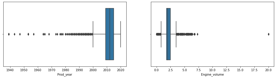
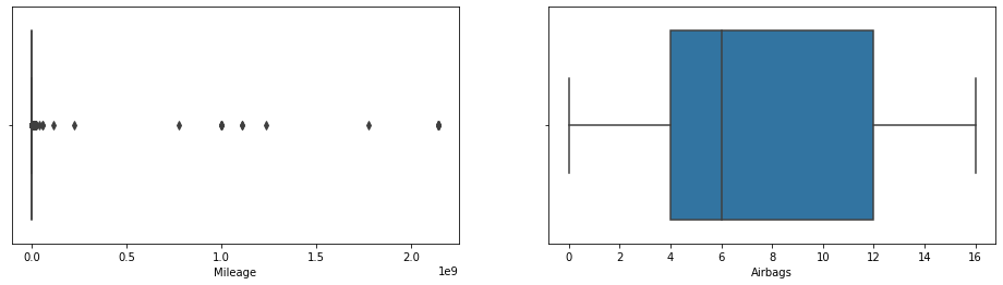
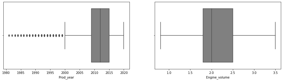
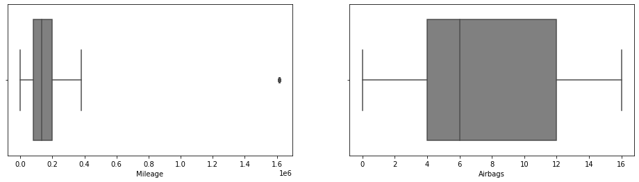
# Detecting outliers in numeric columns
cols=['Price' , 'Levy' , 'Prod_year' , 
'Engine_volume', 'Mileage','Cylinders', 'Doors' , 'Airbags']

cat_cols = ['Price' , 'Levy' , 'Prod_year' , 
'Engine_volume','Mileage', 'Airbags']
i=0
while i < 6:
    fig = plt.figure(figsize=[25,4])
    #ax1 = fig.add_subplot(121)
    #ax2 = fig.add_subplot(122)
    
    #ax1.title.set_text(cat_cols[i])
    plt.subplot(1,3,1)
    sns.boxplot(x=cat_cols[i], data=df)
    i += 1
    
    #ax2.title.set_text(cat_cols[i])
    plt.subplot(1,3,2)
    sns.boxplot(x=cat_cols[i], data=df)
    i += 1
    
    plt.show()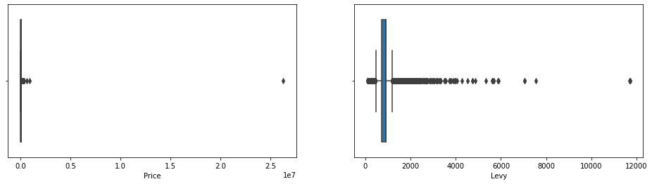

Step_6 Treating Outliers

# Function for imputing outliers in numeric columns
def impute_outliers_IQR(df):

   q1=df.quantile(0.25)

   q3=df.quantile(0.75)

   IQR=q3-q1

   upper = df[~(df>(q3+1.5*IQR))].max()

   lower = df[~(df<(q1-1.5*IQR))].min()

   df = np.where(df > upper,

       df.mean(),

       np.where(

           df < lower,

           df.mean(),

           df

           )

       )

   return df

# Impute outliers in numeric columns
df['Levy'] = impute_outliers_IQR(df['Levy'])
df['Engine_volume'] = impute_outliers_IQR(df['Engine_volume'])
df['Mileage'] = impute_outliers_IQR(df['Mileage'])
df['Price'] = impute_outliers_IQR(df['Price'])

old_cars = df[df['Prod_year']<=1980] #for graph purpose
df = df[df['Prod_year']>1980] #update by droping few entries to improve outlier condition
# Set index to production year
plt.figure(figsize=(20,5))
old_cars.set_index('Prod_year', inplace=True)


# Creating histogram
fig, ax = plt.subplots(figsize =(10, 7))
ax.hist(df['Prod_year'], 
bins = [1980, 1990, 2000, 2010, 2020])
 
# Show plot
plt.xlabel('Production Year')
plt.ylabel('Count')
plt.show()
df.shape

<Figure size 1440x360 with 0 Axes>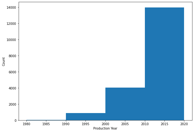

(18900, 18)

# After treatment
cat_cols = ['Price' , 'Levy' , 'Prod_year' ,
 'Engine_volume','Mileage', 'Airbags']
i=0
while i < 6:
    fig = plt.figure(figsize=[25,4])
    #ax1 = fig.add_subplot(121)
    #ax2 = fig.add_subplot(122)
    
    #ax1.title.set_text(cat_cols[i])
    plt.subplot(1,3,1)
    sns.boxplot(x=cat_cols[i], data=df,  
    color='gray')
    i += 1
    
    #ax2.title.set_text(cat_cols[i])
    plt.subplot(1,3,2)
    sns.boxplot(x=cat_cols[i], data=df , 
    color='gray')
    i += 1
    
    plt.show()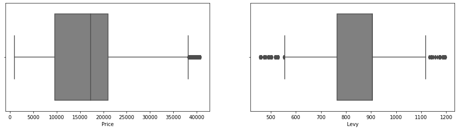

Step_7 Statistics of the dataset

# Summary of the dataset
df.describe()

	Price	Levy	Prod_year	Engine_volume	Mileage	Cylinders	Doors	Airbags
count	18900.000000	18900.000000	18900.000000	18900.000000	1.890000e+04	18900.000000	18900.000000	18900.000000
mean	16141.012594	843.131874	2010.975979	2.161860	2.350861e+05	4.579841	3.932593	6.574074
std	8502.455447	145.360334	5.374868	0.578718	3.782742e+05	1.199205	0.427513	4.319844
min	1000.000000	456.000000	1981.000000	0.800000	1.300000e+01	1.000000	2.000000	0.000000
25%	9565.000000	765.000000	2009.000000	1.800000	7.908000e+04	4.000000	4.000000	4.000000
50%	17249.000000	906.299205	2012.000000	2.000000	1.343860e+05	4.000000	4.000000	6.000000
75%	21005.730841	906.299205	2015.000000	2.500000	2.000000e+05	4.000000	4.000000	12.000000
max	40769.000000	1197.000000	2020.000000	3.500000	1.616358e+06	16.000000	6.000000	16.000000

#for categorical data
df.describe(include=['O']).T

	count	unique	top	freq
Manufacturer	18900	64	HYUNDAI	3729
Model	18900	1578	Prius	1069
Category	18900	11	Sedan	8593
Fuel_type	18900	7	Petrol	9922
Gear_box_type	18900	4	Automatic	13276
Drive_wheels	18900	3	Front	12693
Wheel	18900	2	Left-hand drive	17447
Color	18900	16	Black	4942

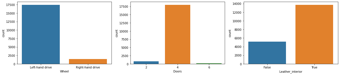
Step_8 Data Visualization

Univariate and Bivariate/Multivariate Analysis and Graphs

cat_cols = ['Fuel_type','Gear_box_type',
'Drive_wheels','Wheel', 'Doors', 'Leather_interior']
i=0
while i < 6:
    fig = plt.figure(figsize=[20,4])
    #ax1 = fig.add_subplot(121)
    #ax2 = fig.add_subplot(122)
    
    #ax1.title.set_text(cat_cols[i])
    plt.subplot(1,3,1)
    sns.countplot(x=cat_cols[i], data=df)
    i += 1
    
    #ax2.title.set_text(cat_cols[i])
    plt.subplot(1,3,2)
    sns.countplot(x=cat_cols[i], data=df)
    i += 1
    
    #ax3.title.set_text(cat_cols[i])
    plt.subplot(1,3,3)
    sns.countplot(x=cat_cols[i], data=df)
    i += 1
    
    plt.show()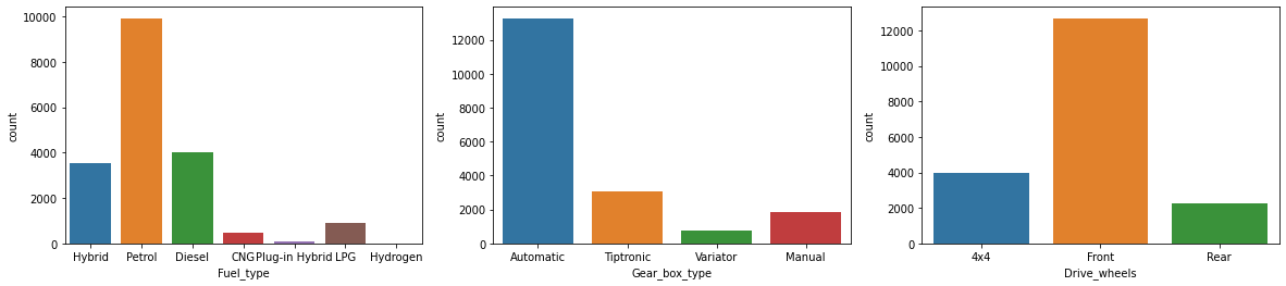

sns.lineplot(data=df, x="Prod_year", y="Price") #drop confidence interval 200,000
plt.ylim(0,50000)
plt.xlabel("Production Year") #drop confidence interval 200,000

Text(0.5, 0, 'Production Year')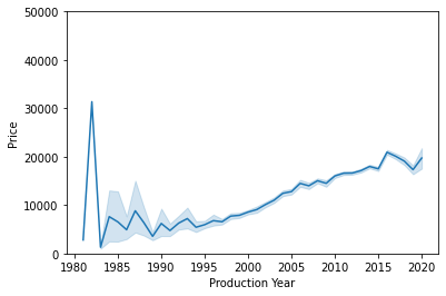

sns.barplot(x="Cylinders", y="Price", data=df)

<AxesSubplot:xlabel='Cylinders', ylabel='Price'>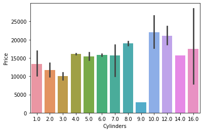

# Checking the normality of the each column
plt.figure(figsize=(10,10))
sns.distplot(df['Levy'])

c:\Users\WASIF\AppData\Local\Programs\Python\Python310\lib\site-packages\seaborn\distributions.py:2619: FutureWarning: `distplot` is a deprecated function and will be removed in a future version. Please adapt your code to use either `displot` (a figure-level function with similar flexibility) or `histplot` (an axes-level function for histograms).
  warnings.warn(msg, FutureWarning)

<AxesSubplot:xlabel='Levy', ylabel='Density'>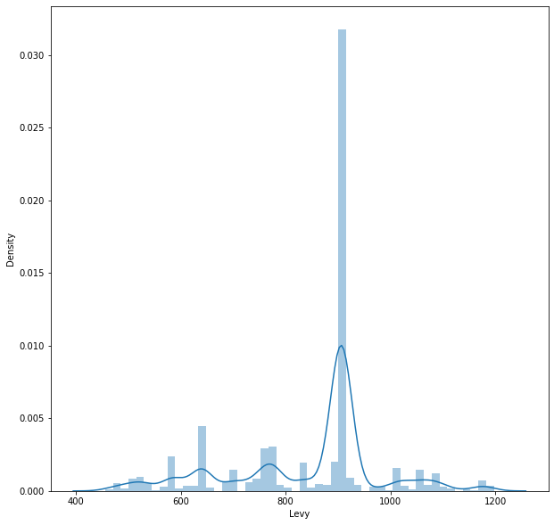

# Normality of mileage column
plt.figure(figsize=(10,10))
sns.distplot(df['Mileage'])

c:\Users\WASIF\AppData\Local\Programs\Python\Python310\lib\site-packages\seaborn\distributions.py:2619: FutureWarning: `distplot` is a deprecated function and will be removed in a future version. Please adapt your code to use either `displot` (a figure-level function with similar flexibility) or `histplot` (an axes-level function for histograms).
  warnings.warn(msg, FutureWarning)

<AxesSubplot:xlabel='Mileage', ylabel='Density'>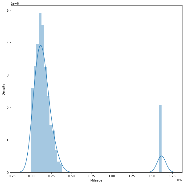

# Normality of price column
plt.figure(figsize=(10,10))
sns.distplot(df['Price'])

c:\Users\WASIF\AppData\Local\Programs\Python\Python310\lib\site-packages\seaborn\distributions.py:2619: FutureWarning: `distplot` is a deprecated function and will be removed in a future version. Please adapt your code to use either `displot` (a figure-level function with similar flexibility) or `histplot` (an axes-level function for histograms).
  warnings.warn(msg, FutureWarning)

<AxesSubplot:xlabel='Price', ylabel='Density'>

# Normal distribution of Production year column
plt.figure(figsize=(10,10))
sns.distplot(df['Prod_year'])

c:\Users\WASIF\AppData\Local\Programs\Python\Python310\lib\site-packages\seaborn\distributions.py:2619: FutureWarning: `distplot` is a deprecated function and will be removed in a future version. Please adapt your code to use either `displot` (a figure-level function with similar flexibility) or `histplot` (an axes-level function for histograms).
  warnings.warn(msg, FutureWarning)

<AxesSubplot:xlabel='Prod_year', ylabel='Density'>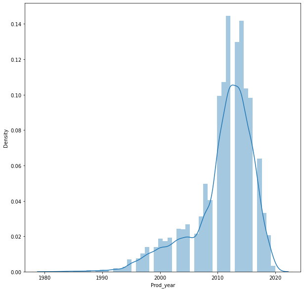

Skewness and kurtosis of the above columns

# Skewness of each column
df.skew()

C:\Users\WASIF\AppData\Local\Temp\ipykernel_1480\546654255.py:2: FutureWarning: Dropping of nuisance columns in DataFrame reductions (with 'numeric_only=None') is deprecated; in a future version this will raise TypeError.  Select only valid columns before calling the reduction.
  df.skew()

Price               0.424448
Levy               -0.586999
Prod_year          -1.305213
Leather_interior   -1.013990
Engine_volume       0.691372
Mileage             3.219546
Cylinders           2.111889
Doors              -2.974352
Airbags             0.085803
Turbo_feature       2.666878
dtype: float64

# kurtois of each column
df.kurt()

C:\Users\WASIF\AppData\Local\Temp\ipykernel_1480\1707974930.py:2: FutureWarning: Dropping of nuisance columns in DataFrame reductions (with 'numeric_only=None') is deprecated; in a future version this will raise TypeError.  Select only valid columns before calling the reduction.
  df.kurt()

Price                0.126193
Levy                 0.136991
Prod_year            1.868845
Leather_interior    -0.971927
Engine_volume       -0.005464
Mileage              8.943932
Cylinders            6.612642
Doors               17.410370
Airbags             -1.331828
Turbo_feature        5.112781
dtype: float64

# Correlation matrix of the dataset
corr = df.corr()

# Heatmap of the correlation matrix of the dataset
plt.figure(figsize=(20,10))
sns.heatmap(corr, annot=True)

<AxesSubplot:>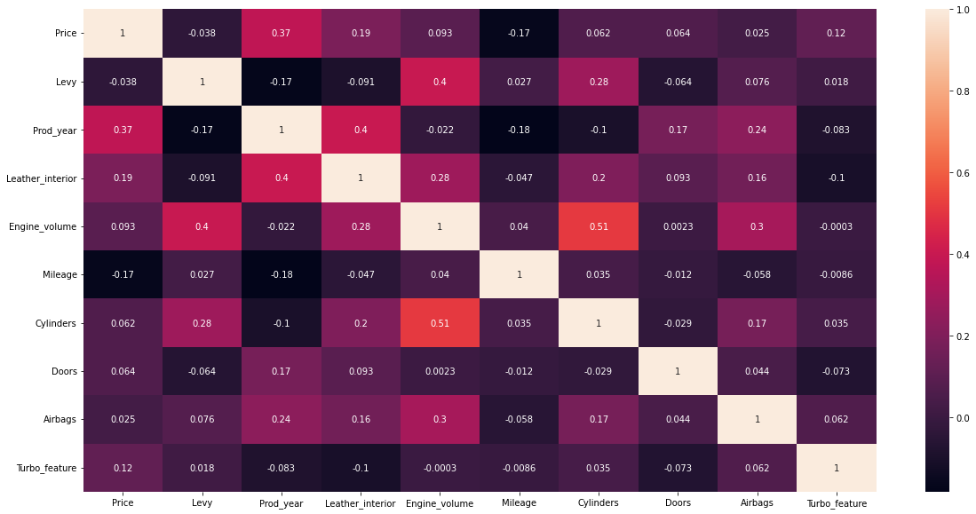

4- Conclusion

Wide variety of manufacturer and car variants are studied having 19237 rows and 18 column in original data set. One column adding no information to data was dropped from the data set. Null values and outlier were treated through mean mutation.

Majority of the cars bought and popular among public are having following features:

- Petrol
- Left hand drive
- Door with 4-cars
- Interior with leather setting
- Gear box having auto-transmission
- Front wheels drive

Based on EDA of data it is observed that price have positive correlation with Turbo Feature, luxury settings like leather interior and production year. It will help in further prediction of prices of cars.

Created in deepnote.com Created in Deepnote

Exploratory Data Analysis on Car prices Prediction Dataset

Submitted by

1- Project Description

A company is planning to build a manufacturing unit. They have gathered car price data from an automobile consulting company of that particular region to understand the factors on which the pricing of cars depends. The company wants to know:

2- Objective

To reach an informed business decision and capturing the market following factors need to carefully studied through EDA:

3- Methodology

Step_1 Importing important libraries

Step_2 Overview of dataset

Import Dataset

Check the Data Shape

Structure of Dataset

Step_3 Cleaning of Data

Rename Columns as a good practice

Dealing with duplicates

Dropping unncessary columns

Now unique value of every column will be checked and listed below those which required treatment. This step is necessary to find out that:

Dealing with null values

Step_4 Type Casting and Replacing Null

Perform type casting to further treat them.

We can see that the percentage of missing values in Levy and Mileage column is low.

In this step we change the data type of each column to its related type.

Treating Enginer_volume Column

Treating door column.

Treating Leather_interior column

We noticed that more than 3500 values of price column is less than $1000. So, we can replace it with the mean of price column.

Step_5 Identification of Outliers

Step_6 Treating Outliers

Step_7 Statistics of the dataset

Step_8 Data Visualization

Skewness and kurtosis of the above columns

Wide variety of manufacturer and car variants are studied having 19237 rows and 18 column in original data set. One column adding no information to data was dropped from the data set. Null values and outlier were treated through mean mutation.

Majority of the cars bought and popular among public are having following features:

Based on EDA of data it is observed that price have positive correlation with Turbo Feature, luxury settings like leather interior and production year. It will help in further prediction of prices of cars.