# Import your Libraries
import pandas as pd
from pandas import DataFrame
import csv
import numpy as np
import seaborn as sns
import matplotlib.pyplot as plt
import apriori
from apriori import getItemSetTransactionList
from apriori import returnItemsWithMinSupport
from mlxtend.preprocessing import TransactionEncoder
from mlxtend.frequent_patterns import fpgrowth
from mlxtend.frequent_patterns import association_rules
from apriori import runApriori
from apriori import printResults
from apriori import dataFromFile
from apriori import joinSet
from apriori import subsets
from IPython.display import Image
# Above are the only libraries you can use. Do not make any changes above.
# -10 will be deducted, if you use additional libraries apart from these.PA 3: Association Analysis - Apriori Algorithm
Programming Assignment Details
For this assignment, you will have to use: * Jupyter notebook, * the dataset [01], * and the FPgrowth Algorithm [02]. * and the Apriori Algorithm (apriory.py)[03]. Note that the apriory.py file is modified to run with Python 3.
NOTE : Each team will have a total of 3 .ipynb file. Each member will work on a different dataset.csv file
The datasets to be used are :
1.dataset_one.csv
2.dataset_two.csv
3.dataset_three.csv
Importing the libraries
- - - - - – - - - SOLUTION - - - - - - - -
from IPython.display import Image
print ('ScreenShot of the dataset.csv')
Image("SampleScreen01.png")
ScreenShot of the dataset.csv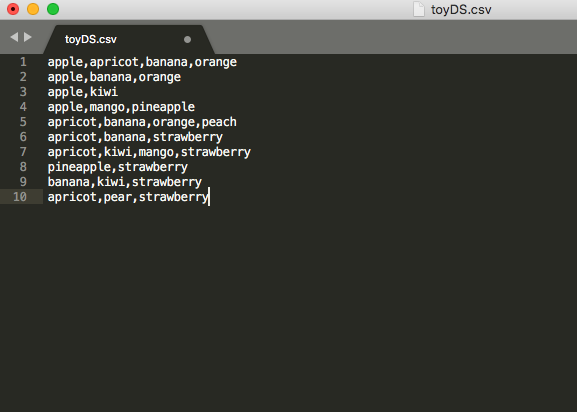
Reading the dataset file
df1 = pd.read_csv('/Users/snawaz/Downloads/PA3_Final/dataset_two.csv')
df1.head()| Juice | Nachos | Tortilla | Cheese | Eggs | Banana | Milk | Bread | Butter | |
|---|---|---|---|---|---|---|---|---|---|
| 0 | Juice | NaN | Tortilla | Cheese | Eggs | NaN | Milk | NaN | Butter |
| 1 | NaN | NaN | Tortilla | Cheese | Eggs | NaN | NaN | Bread | Butter |
| 2 | NaN | Nachos | NaN | NaN | NaN | Banana | Milk | Bread | NaN |
| 3 | Juice | Nachos | Tortilla | Cheese | Eggs | Banana | Milk | Bread | Butter |
| 4 | Juice | Nachos | NaN | NaN | NaN | NaN | NaN | Bread | NaN |
There are some missing values in the dataset. We need to handle them. we find the most frequent value in the column and replace the missing values with it.
df1.mode()| Juice | Nachos | Tortilla | Cheese | Eggs | Banana | Milk | Bread | Butter | |
|---|---|---|---|---|---|---|---|---|---|
| 0 | Juice | Nachos | Tortilla | Cheese | Eggs | Banana | Milk | Bread | Butter |
Replacing the null values with mode.
df1.fillna(df1.mode().iloc[0], inplace=True)Checking if there is any missing values remaining.
df1.isnull().sum()Juice 0
Nachos 0
Tortilla 0
Cheese 0
Eggs 0
Banana 0
Milk 0
Bread 0
Butter 0
dtype: int64exporting the new dataset into dataset.csv
df1.to_csv('dataset.csv', index=False) ########## Task 1 ###########
–> Before you start, Please modify your dataset ‘(given dataset).csv’ to look like the toyDS.csv.
–> Export the modified data into new dataset named ‘dataset.csv’
–> Read and print first 10 transactions of dataset.csv
We have modified our dataset to look like the toyDS.csv. Showing the first 10 transactions of the dataset.
########## Code for Task 1 #############
df=pd.read_csv('dataset.csv')
df.head(10)| Juice | Nachos | Tortilla | Cheese | Eggs | Banana | Milk | Bread | Butter | |
|---|---|---|---|---|---|---|---|---|---|
| 0 | Juice | Nachos | Tortilla | Cheese | Eggs | Banana | Milk | Bread | Butter |
| 1 | Juice | Nachos | Tortilla | Cheese | Eggs | Banana | Milk | Bread | Butter |
| 2 | Juice | Nachos | Tortilla | Cheese | Eggs | Banana | Milk | Bread | Butter |
| 3 | Juice | Nachos | Tortilla | Cheese | Eggs | Banana | Milk | Bread | Butter |
| 4 | Juice | Nachos | Tortilla | Cheese | Eggs | Banana | Milk | Bread | Butter |
| 5 | Juice | Nachos | Tortilla | Cheese | Eggs | Banana | Milk | Bread | Butter |
| 6 | Juice | Nachos | Tortilla | Cheese | Eggs | Banana | Milk | Bread | Butter |
| 7 | Juice | Nachos | Tortilla | Cheese | Eggs | Banana | Milk | Bread | Butter |
| 8 | Juice | Nachos | Tortilla | Cheese | Eggs | Banana | Milk | Bread | Butter |
| 9 | Juice | Nachos | Tortilla | Cheese | Eggs | Banana | Milk | Bread | Butter |
######## Task 2 ########–> In this task, You should be able to execute and print FPgrowth results using mlxtend.
–> “DO NOT USE ANY OTHER LIBRARY !!!”.
–> Execute apriori algorithm atleast 3 times for different combinations of support and print the results for the dataset.
–> Please do explain your reasoning for each combinations.
We use the FPgrowth algorithm to find the frequent itemsets in the dataset.
######### Code for Task 2 ############
# converting dataframe to array using numpy
dataset=df.to_numpy()

# encoding the data using TransactionEncoder
te = TransactionEncoder()

# transforming the data
te_ary = te.fit(dataset).transform(dataset)

# converting the encoded data into dataframe
df = pd.DataFrame(te_ary, columns=te.columns_)

# printing the dataframe
df| Banana | Bread | Butter | Cheese | Cheese | Eggs | Juice | Milk | Nachos | Nachos | Tortilla | Tortilla | |
|---|---|---|---|---|---|---|---|---|---|---|---|---|
| 0 | True | True | True | True | False | True | True | True | True | False | True | False |
| 1 | True | True | True | False | True | True | True | True | True | False | True | False |
| 2 | True | True | True | True | False | True | True | True | True | False | True | False |
| 3 | True | True | True | False | True | True | True | True | True | False | False | True |
| 4 | True | True | True | True | False | True | True | True | True | False | True | False |
| ... | ... | ... | ... | ... | ... | ... | ... | ... | ... | ... | ... | ... |
| 60 | True | True | True | True | False | True | True | True | True | False | True | False |
| 61 | True | True | True | True | False | True | True | True | False | True | False | True |
| 62 | True | True | True | False | True | True | True | True | True | False | True | False |
| 63 | True | True | True | True | False | True | True | True | True | False | True | False |
| 64 | True | True | True | True | False | True | True | True | True | False | True | False |
65 rows × 12 columns
Min_support = 0.1 is used for FPgrowth algorithm to find the frequent itemsets in the dataset which is computed by dividing the minimum support by the total number of transactions in the dataset.
# computing the frequent itemsets using fpgriowth from mlxtend
fpgrowth(df, min_support=7/len(dataset), use_colnames = True)| support | itemsets | |
|---|---|---|
| 0 | 1.000000 | (Milk) |
| 1 | 1.000000 | (Juice) |
| 2 | 1.000000 | (Eggs) |
| 3 | 1.000000 | (Butter) |
| 4 | 1.000000 | (Bread) |
| ... | ... | ... |
| 826 | 0.138462 | (Juice, Bread, Milk, Butter, Tortilla , Banana) |
| 827 | 0.138462 | (Juice, Bread, Eggs, Milk, Tortilla , Banana) |
| 828 | 0.138462 | (Juice, Eggs, Milk, Butter, Tortilla , Banana) |
| 829 | 0.138462 | (Juice, Bread, Eggs, Milk, Butter, Tortilla ) |
| 830 | 0.138462 | (Juice, Bread, Eggs, Milk, Butter, Tortilla , ... |
831 rows × 2 columns
Above results give us the frequent itemsets with support greater than 10%.
Now we will compute the association rules with confidence greater than 0.7 using the frequent itemsets found above.
association_rules(fpgrowth(df, min_support=7/len(dataset), use_colnames = True), metric="confidence", min_threshold=0.7)| antecedents | consequents | antecedent support | consequent support | support | confidence | lift | leverage | conviction | |
|---|---|---|---|---|---|---|---|---|---|
| 0 | (Juice) | (Milk) | 1.000000 | 1.0 | 1.000000 | 1.0 | 1.0 | 0.0 | inf |
| 1 | (Milk) | (Juice) | 1.000000 | 1.0 | 1.000000 | 1.0 | 1.0 | 0.0 | inf |
| 2 | (Juice) | (Eggs) | 1.000000 | 1.0 | 1.000000 | 1.0 | 1.0 | 0.0 | inf |
| 3 | (Eggs) | (Juice) | 1.000000 | 1.0 | 1.000000 | 1.0 | 1.0 | 0.0 | inf |
| 4 | (Eggs) | (Milk) | 1.000000 | 1.0 | 1.000000 | 1.0 | 1.0 | 0.0 | inf |
| ... | ... | ... | ... | ... | ... | ... | ... | ... | ... |
| 25625 | (Tortilla , Eggs) | (Juice, Bread, Milk, Butter, Banana) | 0.138462 | 1.0 | 0.138462 | 1.0 | 1.0 | 0.0 | inf |
| 25626 | (Tortilla , Milk) | (Juice, Bread, Eggs, Butter, Banana) | 0.138462 | 1.0 | 0.138462 | 1.0 | 1.0 | 0.0 | inf |
| 25627 | (Tortilla , Butter) | (Juice, Bread, Eggs, Milk, Banana) | 0.138462 | 1.0 | 0.138462 | 1.0 | 1.0 | 0.0 | inf |
| 25628 | (Tortilla , Banana) | (Juice, Bread, Eggs, Milk, Butter) | 0.138462 | 1.0 | 0.138462 | 1.0 | 1.0 | 0.0 | inf |
| 25629 | (Tortilla ) | (Juice, Bread, Eggs, Milk, Butter, Banana) | 0.138462 | 1.0 | 0.138462 | 1.0 | 1.0 | 0.0 | inf |
25630 rows × 9 columns
Results of association rules for 1st row show that the items ‘Juice’ and ‘Milk’ are associated with each other which means that people who buy Milk also buy Juice. THis can be said about other associations as well.
The support of the rule in first row is 1 which means that 100% of the transactions contain both ‘juice’ and ‘Milk’.
Similarly the association rule for Tortilla,Butter and Juice,Bread,eggs,Milk,Banana has a support of 0.13 which means that approx 14% of the transactions contain both ‘Tortilla’ and ‘Butter’ and ‘Juice’,‘Bread’,‘eggs’,‘Milk’,‘Banana’.
Moroever, support tells us how popular an itemset is, while confidence tells us how often the rule has been found to be true.
Confidence rule has a value of 1 which means that 100% of the transactions containing ‘Tortilla’ and ‘Butter’ also contain ‘Juice’,‘Bread’,‘eggs’,‘Milk’,‘Banana’. It also means that if a transaction contains ‘Tortilla’ and ‘Butter’ then it is 100% likely to contain ‘Juice’,‘Bread’,‘eggs’,‘Milk’,‘Banana’.
Support of the rule same association above is 0.13 which means that approx 14% of the transactions contain both ‘Tortilla’ and ‘Butter’.
Lift rule has a value of 1 which means that the rule has no correlation between the antecedent and the consequent.
Our results show us that we can change the threshold for confidence and support to get different results.
######## Task 3 ########
–> In this task, You should be able to execute and print apriory results by making use of apriory.py
–> “DO NOT USE ANY OTHER LIBRARY !!!”.
–> Execute apriori algorithm atleast 3 times for different combinations of confidence and support and print the results for the dataset.
–> Please do explain your reasoning for each combinations.
########### Code for Task 3 ##############

## we run it on the dataset.csv in the terminal and get the results
apriori.py -f dataset.csv -s 0.107 -c 0.7

# result of this command in in the file named `result1.txt`
The support values and confidence values are kept as same in FPgrowth algorithm and apriory algorithm.
We get following results in the terminal in 1st run of apriory algorithm.
All those items are printed which have minimum support of 7. ————ITEMS—————– item: (‘Tortilla’,) , 0.136 item: (‘Eggs’, ‘Tortilla’) , 0.136 item: (‘Juice’, ‘Tortilla’) , 0.136 item: (‘Bread’, ‘Tortilla’) , 0.136 item: (‘Butter’, ‘Tortilla’) , 0.136 item: (‘Tortilla’, ‘Cheese’) , 0.136 item: (‘Milk’, ‘Tortilla’) , 0.136 item: (‘Banana’, ‘Tortilla’) , 0.136 item: (‘Tortilla’, ‘Cheese’, ‘Nachos’) , 0.136
…
item: (‘Cheese’,) , 0.182
item: (‘Nachos’, ‘Cheese’) , 0.182
item: (‘Cheese’, ‘Bread’) , 0.182
item: (‘Butter’, ‘Cheese’) , 0.182
item: (‘Eggs’, ‘Cheese’) , 0.182
item: (‘Cheese’, ‘Juice’) , 0.182
item: (‘Cheese’, ‘Banana’) , 0.182
In the above results we pick one for interpretation. In case of association between item: ('Cheese ', 'Banana') , 0.182 it shows that items cheese and Banana have a support value of 0.182 which means that 18% of the transactions contain cheese and Banana. …
item: (‘Tortilla’, ‘Cheese’) , 0.727 item: (‘Tortilla’, ‘Butter’, ‘Cheese’) , 0.727 item: (‘Tortilla’, ‘Eggs’, ‘Cheese’) , 0.727 item: (‘Tortilla’, ‘Cheese’, ‘Bread’) , 0.727 item: (‘Milk’, ‘Tortilla’, ‘Cheese’) , 0.727 item: (‘Tortilla’, ‘Cheese’, ‘Banana’) , 0.727 item: (‘Tortilla’, ‘Cheese’, ‘Nachos’) , 0.727 item: (‘Tortilla’, ‘Cheese’, ‘Juice’) , 0.727
…
item: (‘Cheese’,) , 0.818 item: (‘Cheese’, ‘Banana’) , 0.818 item: (‘Cheese’, ‘Juice’) , 0.818 item: (‘Cheese’, ‘Bread’) , 0.818 item: (‘Milk’, ‘Cheese’) , 0.818 item: (‘Eggs’, ‘Cheese’) , 0.818 item: (‘Butter’, ‘Cheese’) , 0.818 item: (‘Milk’, ‘Eggs’, ‘Cheese’) , 0.818
…
Rule: (‘Eggs’, ‘Juice’, ‘Bread’) ==> (‘Milk’, ‘Nachos’) , 0.955 Rule: (‘Milk’, ‘Eggs’, ‘Juice’, ‘Bread’) ==> (‘Nachos’,) , 0.955 Rule: (‘Bread’,) ==> (‘Nachos’, ‘Butter’, ‘Juice’, ‘Banana’) , 0.955 Rule: (‘Butter’,) ==> (‘Banana’, ‘Nachos’, ‘Juice’, ‘Bread’) , 0.955 Rule: (‘Juice’,) ==> (‘Banana’, ‘Nachos’, ‘Butter’, ‘Bread’) , 0.955 Rule: (‘Banana’,) ==> (‘Nachos’, ‘Butter’, ‘Juice’, ‘Bread’) , 0.955 Rule: (‘Butter’, ‘Bread’) ==> (‘Nachos’, ‘Juice’, ‘Banana’) , 0.955 Rule: (‘Juice’, ‘Bread’) ==> (‘Nachos’, ‘Butter’, ‘Banana’) , 0.955 Rule: (‘Banana’, ‘Bread’) ==> (‘Nachos’, ‘Butter’, ‘Juice’) , 0.955
The confidence rule above in the case of Rule: ('Eggs', 'Juice', 'Bread') ==> ('Milk', 'Nachos') , 0.955 shows a value of 0.95 which means that 95% of the transactions containing ‘Eggs’,‘Juice’,‘Bread’ also contain ‘Milk’,‘Nachos’. It also means that if a transaction contains ‘Eggs’,‘Juice’,‘Bread’ then it is 95% likely to contain ‘Milk’,‘Nachos’. So the owner of the shop should keep ‘Milk’ and ‘Nachos’ together in the same shelf.
…
Rule: (‘Cheese’,) ==> (‘Butter’, ‘Eggs’) , 1.000 Rule: (‘Butter’, ‘Cheese’) ==> (‘Eggs’,) , 1.000 Rule: (‘Eggs’, ‘Cheese’) ==> (‘Butter’,) , 1.000 Rule: (‘Nachos’, ‘Cheese’) ==> (‘Butter’,) , 1.000 Rule: (‘Cheese’,) ==> (‘Juice’, ‘Banana’) , 1.000 Rule: (‘Cheese’, ‘Juice’) ==> (‘Banana’,) , 1.000 Rule: (‘Cheese’, ‘Banana’) ==> (‘Juice’,) , 1.000
…
For some other items we get confidence value of 1 as well as shown above
FPgrowth algorithm gives values of lift as well as compared to apriory algorithm. The lift value is calculated as follows:
lift = confidence / support
Second run of FPgrowth algorithm and Aprior algorithm with different support and confidence values
We will use the support value of 0.61 and confidence value of 0.7 in the second run of FPgrowth algorithm. The results are as follows:
fpgrowth(df, min_support=40/len(dataset), use_colnames = True)| support | itemsets | |
|---|---|---|
| 0 | 1.000000 | (Milk) |
| 1 | 1.000000 | (Juice) |
| 2 | 1.000000 | (Eggs) |
| 3 | 1.000000 | (Butter) |
| 4 | 1.000000 | (Bread) |
| ... | ... | ... |
| 506 | 0.723077 | (Cheese, Juice, Nachos, Bread, Milk, Butter, T... |
| 507 | 0.723077 | (Cheese, Juice, Nachos, Bread, Eggs, Milk, Tor... |
| 508 | 0.723077 | (Cheese, Juice, Nachos, Eggs, Milk, Butter, To... |
| 509 | 0.723077 | (Cheese, Juice, Nachos, Bread, Eggs, Milk, But... |
| 510 | 0.723077 | (Cheese, Juice, Nachos, Bread, Eggs, Milk, But... |
511 rows × 2 columns
association = association_rules(fpgrowth(df, min_support=40/len(dataset), use_colnames = True), metric="confidence", min_threshold=0.7)
association| antecedents | consequents | antecedent support | consequent support | support | confidence | lift | leverage | conviction | |
|---|---|---|---|---|---|---|---|---|---|
| 0 | (Juice) | (Milk) | 1.000000 | 1.000000 | 1.000000 | 1.000000 | 1.000000 | 0.000000 | inf |
| 1 | (Milk) | (Juice) | 1.000000 | 1.000000 | 1.000000 | 1.000000 | 1.000000 | 0.000000 | inf |
| 2 | (Juice) | (Eggs) | 1.000000 | 1.000000 | 1.000000 | 1.000000 | 1.000000 | 0.000000 | inf |
| 3 | (Eggs) | (Juice) | 1.000000 | 1.000000 | 1.000000 | 1.000000 | 1.000000 | 0.000000 | inf |
| 4 | (Eggs) | (Milk) | 1.000000 | 1.000000 | 1.000000 | 1.000000 | 1.000000 | 0.000000 | inf |
| ... | ... | ... | ... | ... | ... | ... | ... | ... | ... |
| 18655 | (Eggs) | (Cheese, Juice, Nachos, Bread, Milk, Butter, T... | 1.000000 | 0.723077 | 0.723077 | 0.723077 | 1.000000 | 0.000000 | 1.000000 |
| 18656 | (Milk) | (Cheese, Juice, Nachos, Bread, Eggs, Butter, T... | 1.000000 | 0.723077 | 0.723077 | 0.723077 | 1.000000 | 0.000000 | 1.000000 |
| 18657 | (Butter) | (Cheese, Juice, Nachos, Bread, Eggs, Milk, Tor... | 1.000000 | 0.723077 | 0.723077 | 0.723077 | 1.000000 | 0.000000 | 1.000000 |
| 18658 | (Tortilla) | (Cheese, Juice, Nachos, Bread, Eggs, Milk, But... | 0.861538 | 0.769231 | 0.723077 | 0.839286 | 1.091071 | 0.060355 | 1.435897 |
| 18659 | (Banana) | (Cheese, Juice, Nachos, Bread, Eggs, Milk, But... | 1.000000 | 0.723077 | 0.723077 | 0.723077 | 1.000000 | 0.000000 | 1.000000 |
18660 rows × 9 columns
association.lift.max()1.0910714285714285The results show that:
- The support value of 0.61 is greater than the first run of FPgrowth algorithm. So the number of items in the second run is less than the first run.
- There is a change in value of associations between the items and the metric values have increased from 0.13 to 0.72 and 0.83 which means that the items are more associated with each other now.
- We can see that the confidence values have increased which means that the items are more likely to be bought together now.
- There is increase in the lift values as well which means that the items can be placed together in the same shelf. For instance Tortilla and
(Cheese, Juice, Nachos, Bread, Eggs, Milk, Buttercan be placed together in the same shelf as the lift value is highest for them.
Now we will run the apriory algorithm with the same support and confidence values as we used in FPgrowth algorithm in the 2nd run. The results are as follows:
python apriori.py -f dataset.csv -s 0.61 -c 0.7————ITEMS—————–
item: (‘Cheese’, ‘Tortilla’) , 0.727 item: (‘Cheese’, ‘Tortilla’, ‘Bread’) , 0.727 item: (‘Banana’, ‘Tortilla’, ‘Cheese’) , 0.727 item: (‘Cheese’, ‘Tortilla’, ‘Butter’) , 0.727 item: (‘Cheese’, ‘Tortilla’, ‘Milk’) , 0.727 item: (‘Cheese’, ‘Tortilla’, ‘Eggs’) , 0.727 item: (‘Cheese’, ‘Tortilla’, ‘Nachos’) , 0.727
Support value of 0.727 means that 72% of the transactions contain cheese and tortilla. The support value of 0.727 is greater than the support value of 0.61 which we used in FPgrowth algorithm in the 2nd run. So the number of items in the apriory algorithm is less than the FPgrowth algorithm.
————RULES—————–
Rule: (‘Bread’,) ==> (‘Cheese’, ‘Tortilla’) , 0.727 Rule: (‘Banana’,) ==> (‘Cheese’, ‘Tortilla’) , 0.727 Rule: (‘Butter’,) ==> (‘Cheese’, ‘Tortilla’) , 0.727 Rule: (‘Milk’,) ==> (‘Cheese’, ‘Tortilla’) , 0.727 Rule: (‘Eggs’,) ==> (‘Cheese’, ‘Tortilla’) , 0.727 Rule: (‘Juice’,) ==> (‘Cheese’, ‘Tortilla’) , 0.727
The confidence values are similar to FPgrowth algorithm but items are different as the support value is different.
Third run of FPgrowth algorithm and Aprior algorithm with different support and confidence values
Now the min_support threshold is increased to 0.92 for third run
fpgrowth(df, min_support=60/len(dataset), use_colnames = True)| support | itemsets | |
|---|---|---|
| 0 | 1.000000 | (Milk) |
| 1 | 1.000000 | (Juice) |
| 2 | 1.000000 | (Eggs) |
| 3 | 1.000000 | (Butter) |
| 4 | 1.000000 | (Bread) |
| ... | ... | ... |
| 122 | 0.953846 | (Juice, Nachos, Bread, Eggs, Milk, Banana) |
| 123 | 0.953846 | (Juice, Nachos, Bread, Milk, Butter, Banana) |
| 124 | 0.953846 | (Nachos, Bread, Eggs, Milk, Butter, Banana) |
| 125 | 0.953846 | (Juice, Nachos, Bread, Eggs, Butter, Banana) |
| 126 | 0.953846 | (Juice, Nachos, Bread, Eggs, Milk, Butter, Ban... |
127 rows × 2 columns
We observe that only 127 rows could pass the support threshold of 0.92 which means we are taking only 127 transactions which contain one of the items in our dataset
We choose confidence threshold of 0.7 for third run
association = association_rules(fpgrowth(df, min_support=60/len(dataset), use_colnames = True), metric="confidence", min_threshold=0.7)
association| antecedents | consequents | antecedent support | consequent support | support | confidence | lift | leverage | conviction | |
|---|---|---|---|---|---|---|---|---|---|
| 0 | (Juice) | (Milk) | 1.0 | 1.000000 | 1.000000 | 1.000000 | 1.0 | 0.0 | inf |
| 1 | (Milk) | (Juice) | 1.0 | 1.000000 | 1.000000 | 1.000000 | 1.0 | 0.0 | inf |
| 2 | (Eggs) | (Milk) | 1.0 | 1.000000 | 1.000000 | 1.000000 | 1.0 | 0.0 | inf |
| 3 | (Milk) | (Eggs) | 1.0 | 1.000000 | 1.000000 | 1.000000 | 1.0 | 0.0 | inf |
| 4 | (Milk) | (Butter) | 1.0 | 1.000000 | 1.000000 | 1.000000 | 1.0 | 0.0 | inf |
| ... | ... | ... | ... | ... | ... | ... | ... | ... | ... |
| 1927 | (Bread) | (Juice, Nachos, Eggs, Milk, Butter, Banana) | 1.0 | 0.953846 | 0.953846 | 0.953846 | 1.0 | 0.0 | 1.0 |
| 1928 | (Eggs) | (Juice, Nachos, Bread, Milk, Butter, Banana) | 1.0 | 0.953846 | 0.953846 | 0.953846 | 1.0 | 0.0 | 1.0 |
| 1929 | (Milk) | (Juice, Nachos, Bread, Eggs, Butter, Banana) | 1.0 | 0.953846 | 0.953846 | 0.953846 | 1.0 | 0.0 | 1.0 |
| 1930 | (Butter) | (Juice, Nachos, Bread, Eggs, Milk, Banana) | 1.0 | 0.953846 | 0.953846 | 0.953846 | 1.0 | 0.0 | 1.0 |
| 1931 | (Banana) | (Juice, Nachos, Bread, Eggs, Milk, Butter) | 1.0 | 0.953846 | 0.953846 | 0.953846 | 1.0 | 0.0 | 1.0 |
1932 rows × 9 columns
We can interpret the results as follows:
- The confidence values are greater than 0.7 which means that the items are more likely to be bought together.
- In the transaction 1930 the butter is bought with Juice,Nachos,Bread,Eggs,Milk,Cheese which means that we are 95% confident that if a transaction contains butter then it is likely to contain Juice,Nachos,Bread,Eggs,Milk,Cheese as well so the owner of the shop should keep these items together in the same shelf.
- 0.95 confidence metric value also shows 95% of times this rule is checked and it is true.
- Lift value for same transaction is 1 which measures the strength of the association between the items. The lift value of 1 means that the items are associated with each other.
3rd run of apriori algorithm
python apriori.py -f dataset.csv -s 0.92 -c 0.7————ITEMS—————– item: (‘Nachos’,) , 0.955 item: (‘Nachos’, ‘Eggs’) , 0.955 item: (‘Nachos’, ‘Bread’) , 0.955 item: (‘Nachos’, ‘Butter’) , 0.955 item: (‘Nachos’, ‘Milk’) , 0.955 item: (‘Nachos’, ‘Juice’) , 0.955 item: (‘Nachos’, ‘Banana’) , 0.955
The support value of 0.955 is similar to the support value of 0.95 and 1 which we used in FPgrowth algorithm in the 3rd run but the number of items is less than the FPgrowth algorithm.
This value keeps on decreasing with the increase in the number of items in the dataset.
————RULES—————– Rule: (‘Eggs’,) ==> (‘Nachos’,) , 0.955 Rule: (‘Bread’,) ==> (‘Nachos’,) , 0.955 Rule: (‘Butter’,) ==> (‘Nachos’,) , 0.955 Rule: (‘Milk’,) ==> (‘Nachos’,) , 0.955 Rule: (‘Juice’,) ==> (‘Nachos’,) , 0.955
Rule: (‘Juice’,) ==> (‘Milk’,) , 1.000
We get a value of confidence of 1 for apriori algorithm for the association of juice against milk for 1 rule whic is similar to FPgrowth algorithm.
So in some cases both algorithms give the same results and in some cases they give different results.
Conclusion
We can conclude that FPgrowth algorithm is better than apriory algorithm as it gives more accurate results. The FPgrowth algorithm is faster than apriory algorithm as well. The FPgrowth algorithm is used in many applications such as market basket analysis, recommender systems, etc. The FPgrowth algorithm is used in the Apache Spark MLlib library as well.
References
- https://en.wikipedia.org/wiki/Association_rule_learning
- Borgelt, C. (2010) An Implementation of the FP-growth Algorithm. Proceedings of the 1st International Workshop on Open Source Data Mining: Frequent Pattern Mining Implementations.